Explanation

Background and the reasoning behind how InTerra Studio works — read these to understand the why, not to follow steps.

Why ground control matters

InTerra Studio's GNSS workflow exists for one reason: to give your photogrammetry hard, survey-grade truth on the ground. Without it, even a beautifully-textured 3D model can be drifting — slightly stretched, subtly rotated, or floating at the wrong elevation. Ground control points (GCPs) solve that.

What GCPs do. Photogrammetry reconstructs shape and texture from overlapping images, but on its own it has no inherent sense of real-world scale, orientation, or absolute position. The bundle-adjustment math can produce a visually convincing model that's nevertheless geometrically off. A GCP ties a pixel-level feature in the imagery to a precisely-known coordinate on the ground, forcing the reconstruction to align with a stable geodetic reference frame. Even a small number of well-distributed GCPs dramatically improves accuracy — especially the vertical, which is traditionally the weakest dimension in photogrammetry.

How Studio + SmarTargets streamline it. The traditional approach is to walk the site, shoot each target individually with a roving GNSS receiver, and later match them by hand. Studio with SmarTargets short-circuits that: the target is the GNSS logger. Place it, fly the mission, and let the Datum and Process tabs derive its surveyed coordinate automatically. You can afford more targets, distribute them more effectively, and end up with a stronger, more defensible photogrammetric block.

Why an RTK drone isn't a replacement for GCPs

RTK improves the camera position recorded with each photo, but photogrammetry isn't just stamping coordinates onto images — the reconstruction depends on the geometry between images: tie points, camera calibration, lens distortion, flight dynamics, and the bundle adjustment that stitches everything together. Even with perfect RTK on the drone:

• RTK errors accumulate. Multipath, canopy, urban reflections, brief signal dropouts — all introduce centimeter-to-decimeter-level errors that propagate into systematic distortions (tilted surfaces, bowed elevations, creeping horizontal shifts) across the photogrammetric block. GCPs act as independent checkpoints that expose and correct these biases.
• RTK gives absolute camera position; GCPs give geometric stability. The solver can still deform the block internally even with perfect camera centers, because it's solving for camera orientation, lens parameters, and 3D structure simultaneously. Fixed ground points are "hard stops" that prevent bending or stretching, especially in long corridors, large areas, or terrain with poor texture.
• RTK + GCPs is the gold standard, not RTK vs GCPs. RTK reduces the number of GCPs you need but doesn't eliminate them. A small number of well-placed GCPs dramatically improves accuracy and validates that the RTK solution behaved as expected across the whole project.

The practical takeaway: even if your drone is RTK-equipped, a handful of SmarTargets gives you a far stronger, more defensible final dataset than RTK alone. Studio's job is the ground-control side of that equation — it processes your SmarTargets into GCPs and does not ingest or correct the drone's own positions. An RTK/PPK drone — one that records a corrected, survey-grade position with each photo — is complementary to that, not something you process here.

Heights: ellipsoidal vs. orthometric

Survey work cares about two kinds of height. Ellipsoidal heights are measured from a smooth mathematical model of the earth (what raw GNSS satellite positioning gives you). Orthometric heights are measured from the geoid — effectively "height above mean sea level" — which is what most engineering and survey deliverables expect. InTerra lets you choose which one your project uses (on Project Information) and handles the conversion for you so your elevation models come out in the frame your client asked for. See the Glossary for the short definitions.

Working in metric or imperial

InTerra is units-aware throughout. You can work in metric or imperial, and controls adapt — for example, the flight-height slider steps by 1 m in metric or 5 ft in imperial, and readouts like ground sample distance show the matching units. Set your preference once and the whole app follows it.

Zero Persistence Computing

How your data is protected. Building a model means sending your imagery to InTerra's cloud processing. Because that imagery is your customers' data — and often sensitive — Studio is built around a principle we call Zero Persistence Computing: your data is processed without being retained on our infrastructure after processing. The outputs you generate — point clouds, orthomosaics, and models — are yours to keep; we don't hold your project outputs after processing, and we don't use your data to train models or build derivative products. Here's what that means in practice.

Dedicated, private machines — not shared storage. When you start a build, InTerra provisions processing machines just for your job. Your photos and the resulting deliverables live only on those dedicated machines while they work, and the machines are destroyed the moment the job finishes. Your data's lifetime equals your job's lifetime. It is never placed in a shared, multi-tenant, or persistent cloud storage bucket where it would linger after the job — a convenience InTerra deliberately gives up precisely so there's never a copy of your imagery sitting in the cloud to explain or worry about.

Encrypted, verified connections end to end. Every connection that carries your imagery or results is encrypted in transit, and — just as importantly — the receiving machine is cryptographically verified before any data is sent. InTerra "pins" the exact identity of each processing machine, so your data can only ever travel to the genuine machine provisioned for your job and can't be silently intercepted or redirected to an impostor. This protection covers the whole path: from the application to the coordination service, and across the internal hops between the processing machines themselves.

Per-job access, automatically revoked. Each job is issued its own access credential that is scoped to that single job and invalidated when the job's machines are torn down. There is no long-lived, shared key that could be reused later.

Why this matters to you. Many of InTerra's customers — state DOTs, engineering firms, surveyors working under confidentiality obligations — can't have their survey imagery resting in a general-purpose cloud store. With InTerra, you can tell your client, accurately, that their data is processed on a private machine dedicated to their job, over encrypted and verified connections, and is gone when the job is done. The only practical cost of this design is that if a processing machine has a rare mid-job failure, InTerra re-sends the imagery to a fresh machine rather than keeping a stored copy around — a few extra minutes on a job measured in hours, in exchange for never leaving your data where it shouldn't be.

Questions you — or your client — might ask.

• Where exactly does my imagery go during a build? To a processing machine provisioned specifically for your job, reached over an encrypted, identity-verified connection. It is not uploaded to a general-purpose or shared cloud storage service.
• Is my data stored anywhere after the job finishes? No. The machines that held it are destroyed when the job ends, and your imagery is never copied into a persistent shared store. Your finished deliverables are downloaded back into your own project folder on your computer.
• Could someone intercept my data in transit? Connections are encrypted, and InTerra verifies the exact identity of the receiving machine before sending — so your data can only travel to the genuine machine for your job, not to an impostor, and can't be read in flight.
• Does InTerra keep my imagery for analytics, training, or to build derivative products? No — there's no retained copy to keep; the machine your data lived on is torn down after the job, and your data is never used to train models or build derivative products.
• What happens if processing fails partway through? InTerra re-sends your imagery to a fresh dedicated machine rather than reusing a stored copy (because there isn't one). It costs a little time on a rare failure, by design.

Getting accurate results

A few habits consistently produce better, cheaper, more accurate jobs.

• Get the foundation right first. An accurate boundary and the correct coordinate system / height type on Project Information prevent a whole class of "the model is in the wrong place / wrong height" problems downstream. Fixing them early is cheap; fixing them late means re-checking everything that depended on them.
• Plan your GSD, don't discover it. On Pre-Flight, choose the height that delivers the GSD your deliverable actually requires. Flying needlessly low multiplies your photo count, processing time, and credit cost for detail no one asked for.
• Place control with good geometry. Spread ground targets toward the edges and corners of the site, and pick high-contrast colors with Suggest Colors. Well-distributed, easy-to-see control is the single biggest lever on absolute accuracy.
• Enter a known base position when accuracy is absolute. On Datum, an approximate base position gives you a relatively-accurate model referenced to an approximate point. A surveyed known position is what makes the result absolutely accurate.
• Cull before you build. On Flight Review, drop redundant and out-of-boundary photos. You keep the coverage you need and cut processing time and credits on the photos that only repeat what their neighbors already saw.
• Tag GCPs in several photos and trust the colors. In Target Finder, more well-spread picks per point make a stronger solution; let the green / yellow / red quality tiers steer you to the picks worth re-checking.
• Only generate the outputs you need. Each output on Build Model adds time and credits. Run again later if you need more — it's cheaper than always producing everything.
• Use the Prediction as a pre-flight check for the build. Glance at the estimated GSD, area, counts, download size, and credits before you start, so a surprise (a huge area, a download that won't fit) shows up before you spend the run.
• Save often. Press Ctrl+S after meaningful changes so your boundary, settings, and control-point work are safely written to the project.

Processing reference

Background reading for what's going on under the hood when InTerra Studio turns raw GNSS observations into a corrected ground-control point. You don't need any of this to use Studio — the Process tab will run the math and report back numbers. This section is for when you want to know what those numbers actually mean.

---

The ECEF coordinate frame

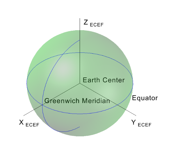
Earth-Centered, Earth-Fixed (ECEF): X points to the equator at the Greenwich Meridian, Y to 90° E along the equator, Z to the North Pole.

The Earth-Centered, Earth-Fixed (ECEF) coordinate system is a global, geocentric Cartesian reference frame used widely in geodesy, GNSS, and 3D spatial computation. Positions are expressed as X, Y, Z in metres measured from the Earth's centre of mass.

ECEF is Earth-fixed — the axes rotate with the planet. As the Earth turns, the coordinate grid turns with it, so any point on the surface keeps a nearly constant coordinate value (aside from tectonic motion and datum updates).

Axis definitions.

• X axis — from the Earth's centre toward the intersection of the equator and the prime meridian (0° latitude, 0° longitude).
• Y axis — from the Earth's centre toward 90° east longitude along the equator.
• Z axis — from the Earth's centre toward the North Pole (90° latitude).

Together these axes form a right-handed coordinate system.

Key characteristics.

• Global and continuous — one planet-wide frame, no zone discontinuities and no projection seams.
• Cartesian — linear units (metres), so vector math, distance calculations, and 3D transformations are straightforward.
• Datum-dependent — in Studio, ECEF coordinates are tied to WGS 84.
• Foundation for local frames — East-North-Up (ENU) and similar local tangent-plane systems are derived from ECEF at a chosen reference point. Variance in Studio is reported in ENU (see below).

Why ECEF. It's the native coordinate system for GNSS satellites and many geospatial algorithms. It avoids the distortions and singularities of latitude/longitude (no pole problem, no antimeridian wrap-around) and enables precise 3D computation, transformation, and integration with inertial sensors.

---

WGS 84 and transformations

Studio's GNSS pipeline operates natively in the WGS 84 reference frame. All incoming GNSS positions, ECEF coordinates, and derived ENU values are initially expressed in WGS 84 so the entire chain is consistent with what the satellites broadcast.

When a project's coordinate reference system is something else — a national grid, a state-plane zone, a projected system, or a local engineering datum — Studio applies the appropriate transformation from WGS 84 into the target system at the output stage. Those transformations can include:

• Helmert (7-parameter) datum shifts;
• grid-based corrections where authoritative grids are available;
• projection steps (UTM, State Plane, national mapping grids).

The raw GNSS data stays tied to WGS 84; only the transformed output is expressed in the requested coordinate system. Every computation starts from a single globally-recognized reference, while still producing the regional / project-specific coordinates you actually need to deliver.

---

Variance

Variance is the headline quality number Studio reports for each processed target — how tightly the corrected position clustered over the observation window. Smaller variance means a more stable solution with less positional scatter; larger variance means more noise, multipath, or degraded correction quality.

How it's computed. For each axis (East, North, Up) of the local tangent-plane ENU frame, Studio uses the unbiased sample variance:

        1    n
σ²  =  ───  Σ ( xᵢ − x̄ )²
       n−1  i=1

where xᵢ is the ENU value at observation epoch i, x̄ is the mean for that axis, and n is the number of filtered solutions kept after quality / ratio / satellite / time-trim filters in Process.

Units. Variance is naturally in m². Studio reports in mm² by multiplying by 10⁶ (since a millimetre is a thousandth of a metre, a square millimetre is one-millionth of a square metre):

e_mm²  =  e_m²  ×  10⁶

Sensitivity to sample size. Variance does not depend on the number of observations — it reflects only the scatter. More observations just produce a more reliable estimate of the true variance; they don't shrink it. Long survey sessions don't "average down" a noisy unit.

Typical ranges (mm²). Expected performance for survey-grade RTK / PPK receivers. Use these as a sanity check on what the Process tab reports.

Quality	Horizontal (East, North)	Vertical (Up)
Excellent	1 – 25 mm² (~1 – 5 mm scatter)	4 – 100 mm² (~2 – 10 mm scatter)
Good	25 – 100 mm² (~5 – 10 mm)	100 – 400 mm² (~10 – 20 mm)
Acceptable	100 – 400 mm² (~10 – 20 mm)	400 – 1200 mm² (~20 – 35 mm)
Poor	> 400 mm² (> 20 mm)	> 1200 mm² (> 35 mm)

These are practical benchmarks for evaluating solution stability — the lower the values, the tighter the cluster, the higher the confidence in the measurement quality.