Tutorial — A full survey, start to finish

This walks the entire InTerra Studio workflow end to end — from an empty project to an explorable 3D model — using a real sample survey of a Jacksonville, FL site. The only thing you won't do is fly the drone: the photos and field GNSS logs are already captured for you.

You don't need a drone, field hardware, or any cloud credits. The final model build is simulated for the tutorial so it runs instantly and costs nothing; on a real job that step uploads your photos and processes them in the cloud.

Plan for about 20 minutes. Follow it straight through and you'll finish with corrected ground control, a culled photo set, tagged control points, and a 3D model you can measure — the whole shape of a survey-grade job.

Step 1 — Create the project (Project Information)

Start InTerra Studio. It opens on the Start window — recent projects on the left, and the panel on the right for starting a new one.

1. On the Start window, click Create a new project.

2. In the Create InTerra Project window, set the Project Name to Jacksonville HD. InTerra uses the name for the project folder too, created under your Root folder. Click Create.

   The name only has to be close — matching isn't case-sensitive and doesn't have to be exact, so jacksonville hd or JAX HD will do. That's what tells InTerra this is the tutorial project and triggers the sample-data offer in the next step.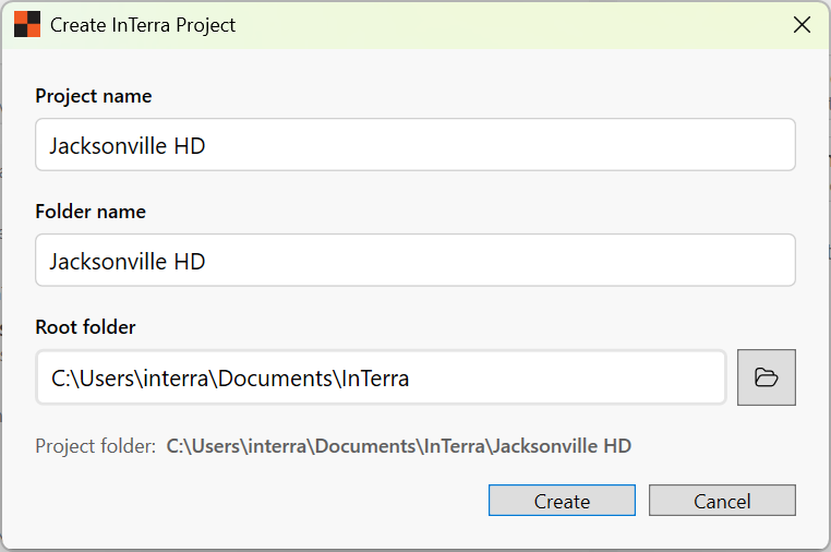

   

   Screenshot: the Create InTerra Project window, with the project name, folder name, and root folder set — the project folder it will create is shown underneath.

3. Because the name matches the tutorial, InTerra offers to download the sample dataset — the field .ubx logs and the drone images. Say yes; it's a one-time download, cached locally afterward. The project then opens in Studio with Jacksonville HD shown at the top of the window.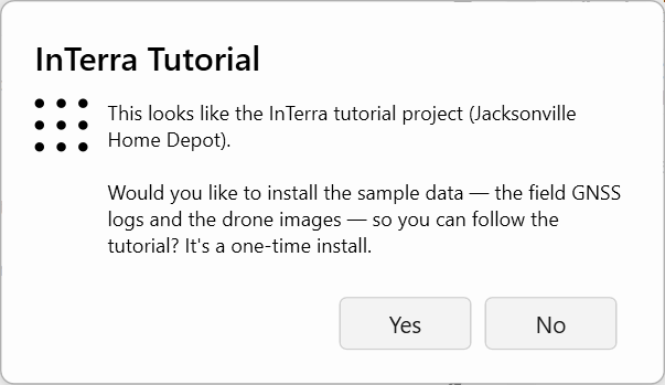

   

   Screenshot: InTerra recognizes the tutorial project and offers to install the sample data — the field GNSS logs and the drone images.

4. In the Details card, set the site address to 9600 San Jose Blvd, Jacksonville, FL 32257. You don't have to type the whole thing — start typing 9600 San J, pick the full address from the top of the suggestions, and the map geocodes and zooms to the site.

5. With the location set, the Location fields fill in automatically — and so does the Coordinate system: InTerra defaults this site to Florida East (ftUS) with orthometric heights on NAVD88 (GEOID18). That's the right system here, so leave it. Setting the address first is what lets InTerra pick the system for you — see Reference → Project Information.

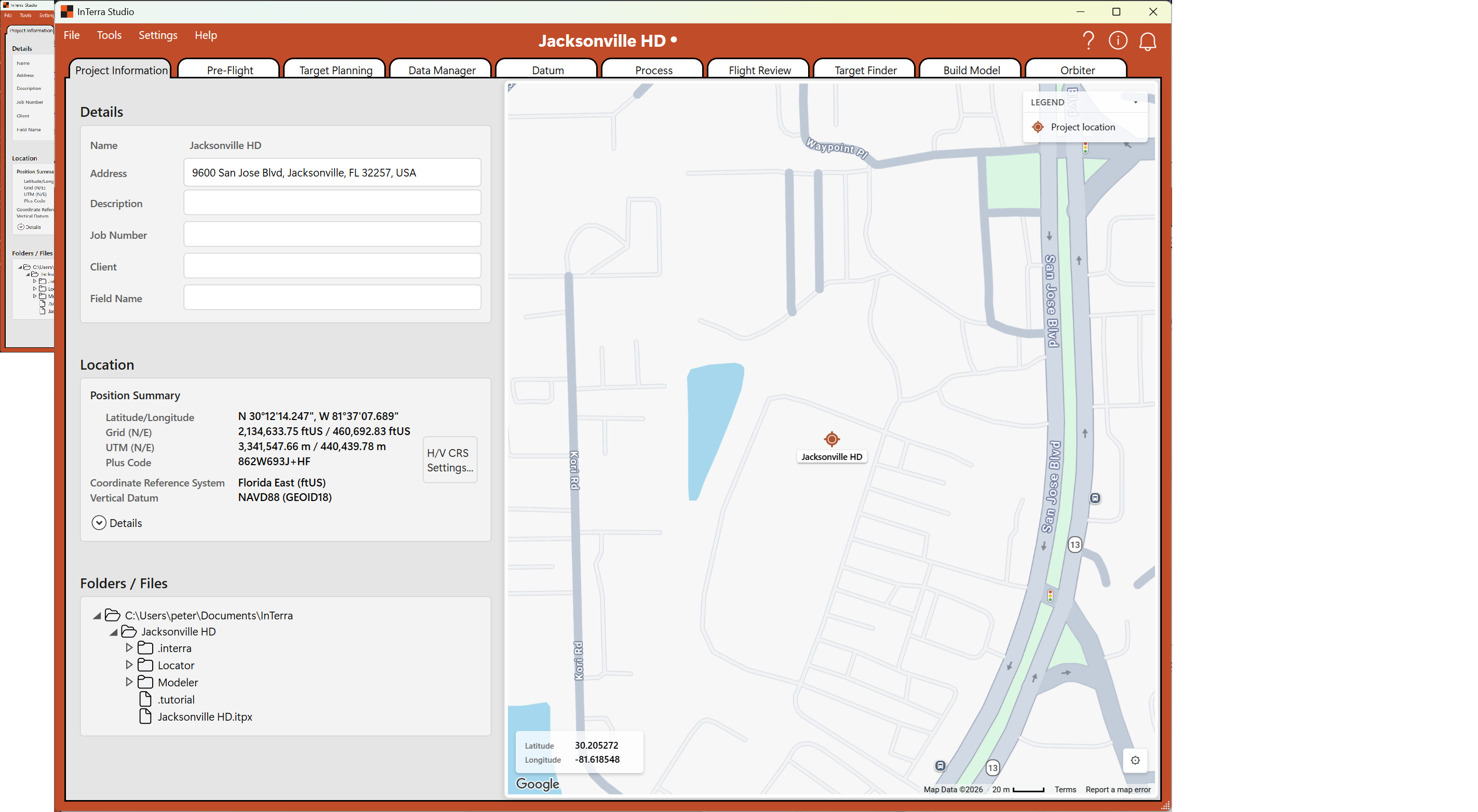
Screenshot: Project Information with the site located — the address geocoded, the Position Summary filled in, and the coordinate system defaulted to Florida East (ftUS) on NAVD88 (GEOID18).

Your project now has a name, a location, and the correct coordinate system.

Notice the dot after the project name at the top of the window. That's InTerra telling you the project has unsaved changes — it appears whenever you change something and clears when you save (File → Save Project, or Ctrl+S). It's worth saving here.

A note on planning — Pre-Flight & Target Planning

On a real job, before you fly you'd use Pre-Flight to plan the mission (camera, height, ground sample distance) and Target Planning to lay out where your ground targets go. Because this sample is already flown, we skip straight to processing the data that came back — but it's worth knowing those tabs are the front half of the workflow. See Pre-Flight and Target Planning when you plan your own job.

Step 2 — Download the GNSS logs (SmarTarget Manager)

When a flight is done, you connect the Datum receiver and the SmarTarget units to your computer with the supplied USB cables and 7-port hub and download their GNSS logs directly into Studio, charge the units for the next mission. This can happen on a laptop in the field right after the flight, or back in the office — whichever fits your workflow. The on-unit SD cards hold hundreds of missions, so you only need to download when you're ready to process — not between flights.

For the tutorial you don't need any hardware: InTerra supplies the units, pre-loaded with the sample logs, so you can walk the real download.

Watch it first (1:50): InTerra SmarTarget Charging & Data Download — how the units charge and how the logs come off, on real hardware.

Open Tools → SmarTarget Manager.

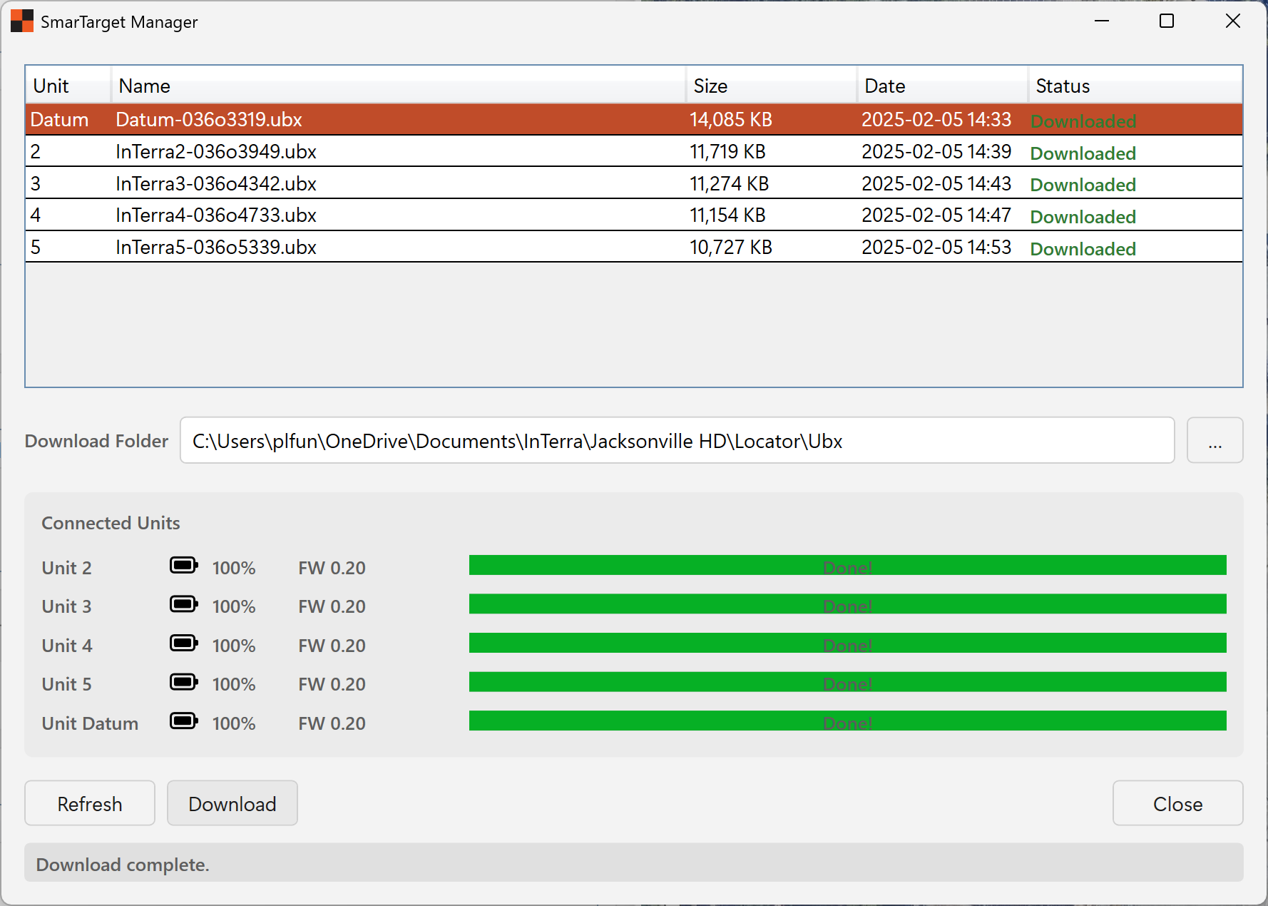
Screenshot: the SmarTarget Manager with the five tutorial units connected — the Datum unit and InTerra2 through InTerra5 — and their logs selected for download.

1. The grid lists the connected units and their logs — the Datum unit and four targets (InTerra2 through InTerra5), five logs in all. Select all five.
2. Click Download at the bottom of the window. The logs land in the project, ready for the next step. They download instantly in the tutorial; from real units each log is ~10–14 MB and takes about a minute over USB (≈4–5 minutes for all five).

The same window also shows each unit's battery charge and the live download progress, and lets you delete already-downloaded logs from a unit's SD card to free space. See Reference → SmarTarget Manager.

Step 3 — Import the GNSS logs (Data Manager)

Back in the office, Data Manager is where your field GNSS logs become survey-grade reference data: it converts the raw .ubx logs you downloaded in Step 2 to RINEX for processing, and pulls CORS reference files from the NOAA servers.

Open Data Manager.

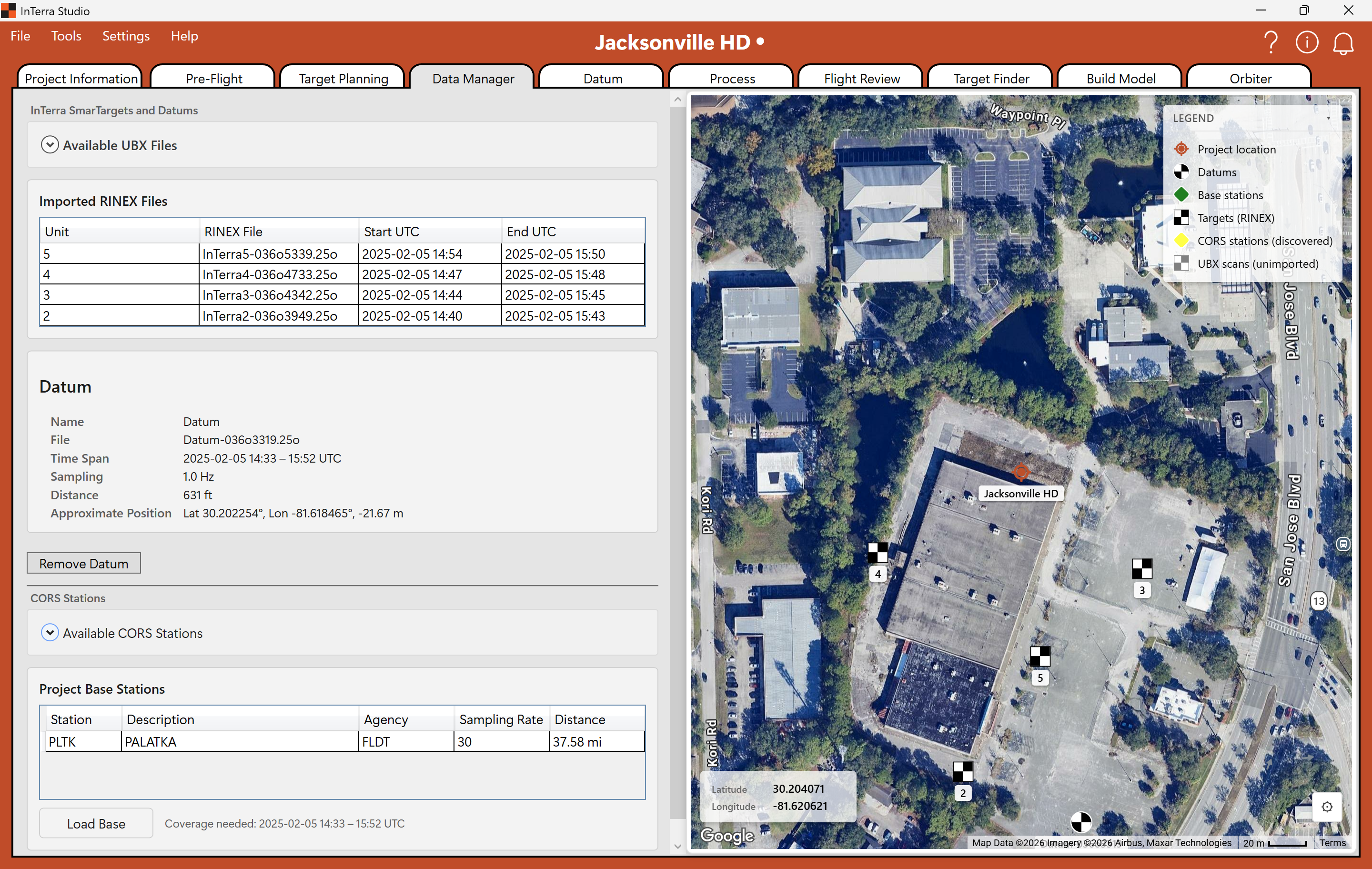
Screenshot: Data Manager with the five tutorial UBX logs added to the project and the PLTK CORS station downloaded — its map diamond green.

1. Under Available UBX Files, InTerra lists the logs it found, sorted by approximate distance from the project location. The same files appear on the map as gray-and-white markers, so you can select from either the grid or the map. The tutorial set is five logs collected at the site on Feb 5, 2025, 275–631 ft from the project location: the Datum log and four SmarTarget units (InTerra2 through InTerra5). Select all five and click Add to project.
2. Typically, the Import Files window asks whether to Move or Copy the logs into the project. For this tutorial it will move the files automatically. You could instead choose Copy so the originals stay in your download folder and you can run the tutorial again. (Move relocates them into the project and removes them from the download folder.)
3. InTerra converts the logs to RINEX and adds them to the project; their map markers turn from gray-and-white to black-and-white.
4. Now bring in the CORS reference. Open Available CORS stations, select PLTK (Palatka — about 38 mi south of the site; zoom out to see its yellow diamond on the map), and click Download and Add. InTerra fetches the PLTK RINEX from NOAA for a window covering the flight. When it's added, the diamond turns green.

Close the Available UBX and Available CORS cards to focus on what's now in the project, and glance at the Base Station info card to confirm the import.

Good moment to save (Ctrl+S) — you've just brought a set of field data into the project, and the dot beside the project name is showing again.

Full detail in Reference → Data Manager.

Step 4 — Set the reference (Datum)

The Datum tab is where you refine the position of the InTerra Datum unit — the base receiver that was logging during the flight. Its raw log gives only an approximate position; processing it against a published reference fixes it precisely.

Open Datum. Because a CORS file and a Datum log are both in the project, InTerra opens ready to process the Datum against the CORS station.

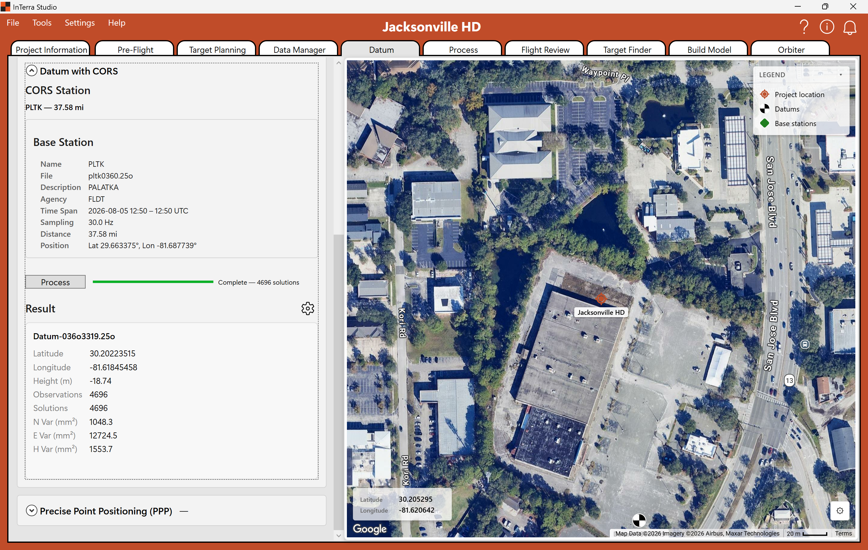
Screenshot: the Datum tab set to process the Datum log against the PLTK CORS station, with the solved position shown.

For this tutorial we anchor the Datum to the PLTK CORS station. This isn't the most accurate option — a surveyed known position on your own base is — but it's the most common real-world setup, and it's how you bring a published reference into a job. (See the how-to guides for processing directly against CORS or with a surveyed known position.)

Click Process to run a PPK solution of the Datum log against PLTK. When it finishes, the Datum's solved lat / lon / height appear — notice they differ from the approximate position it started with. That solved position is now the reference your units are corrected against.

Step 5 — Process the units (Process)

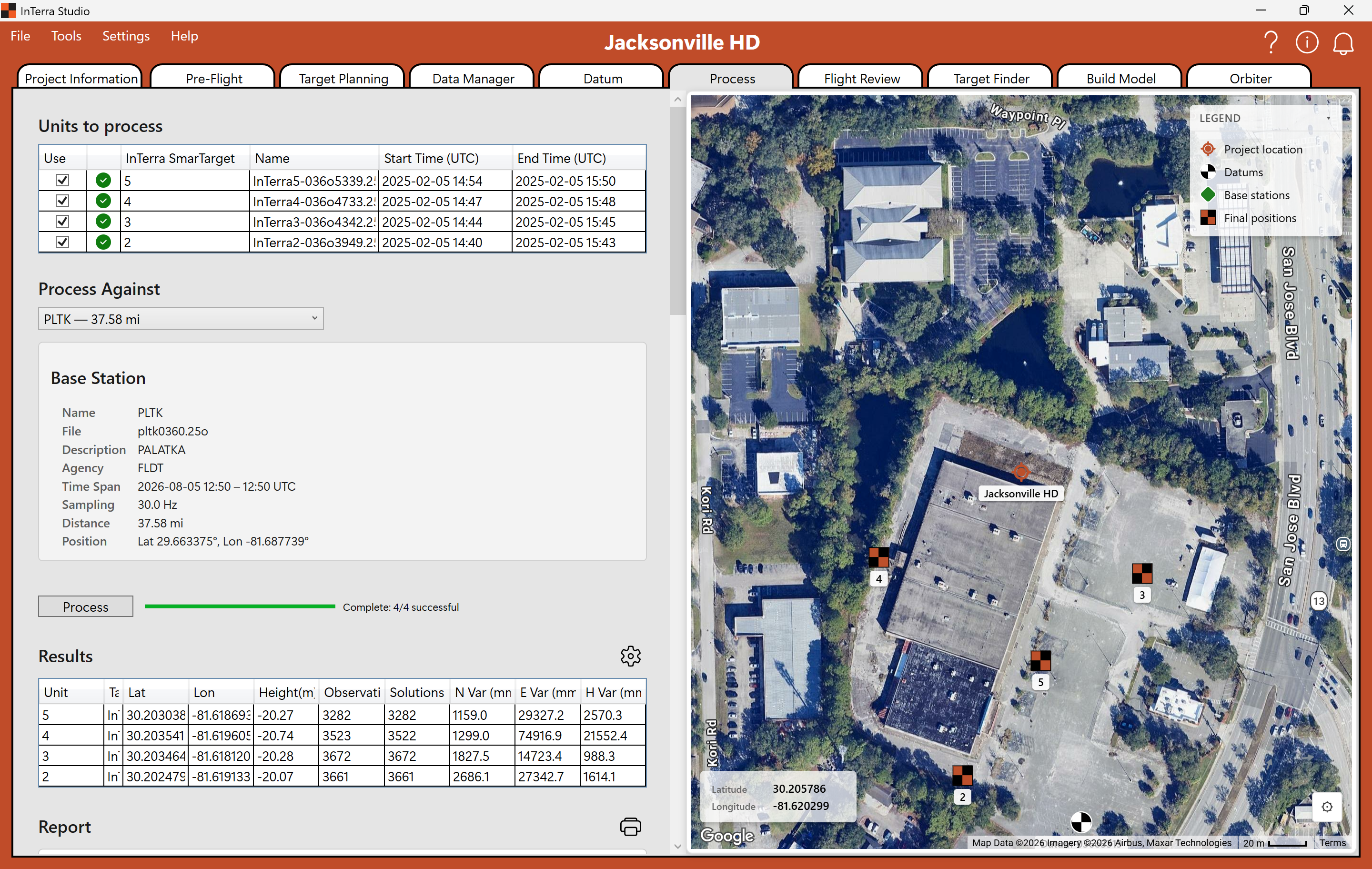
Screenshot: the Process tab after a run — each unit checked, its status settled, and the variance for each corrected position.

Open the Process tab. You'll see your survey units (the targets), each with a Use checkbox and a status column. Make sure the units are checked, set Process against to Datum processed against PLTK, and click Process to run the PPK corrections.

InTerra corrects each unit against the Datum and reports back. Watch the status column settle; each result carries a variance — a measure of how tightly the position resolved (lower is tighter; see Explanation → Variance).

The results here are solid. If you'd like to explore, the gear to the right of Results lets you adjust the Confidence and other factors, and the Measure To dropdown lets you reference the correction differently (try Bottom of Case). Both are optional and will shift the corrected numbers a little — that ripples into the ground control, so your values may end up slightly different from the sample we ship. For the tutorial, either way is fine.

You now have corrected, survey-grade ground control for the site. This is the heart of the whole survey — and on this dataset it's the real thing, not a simulation.

Step 6 — Import your imagery (Flight Review)

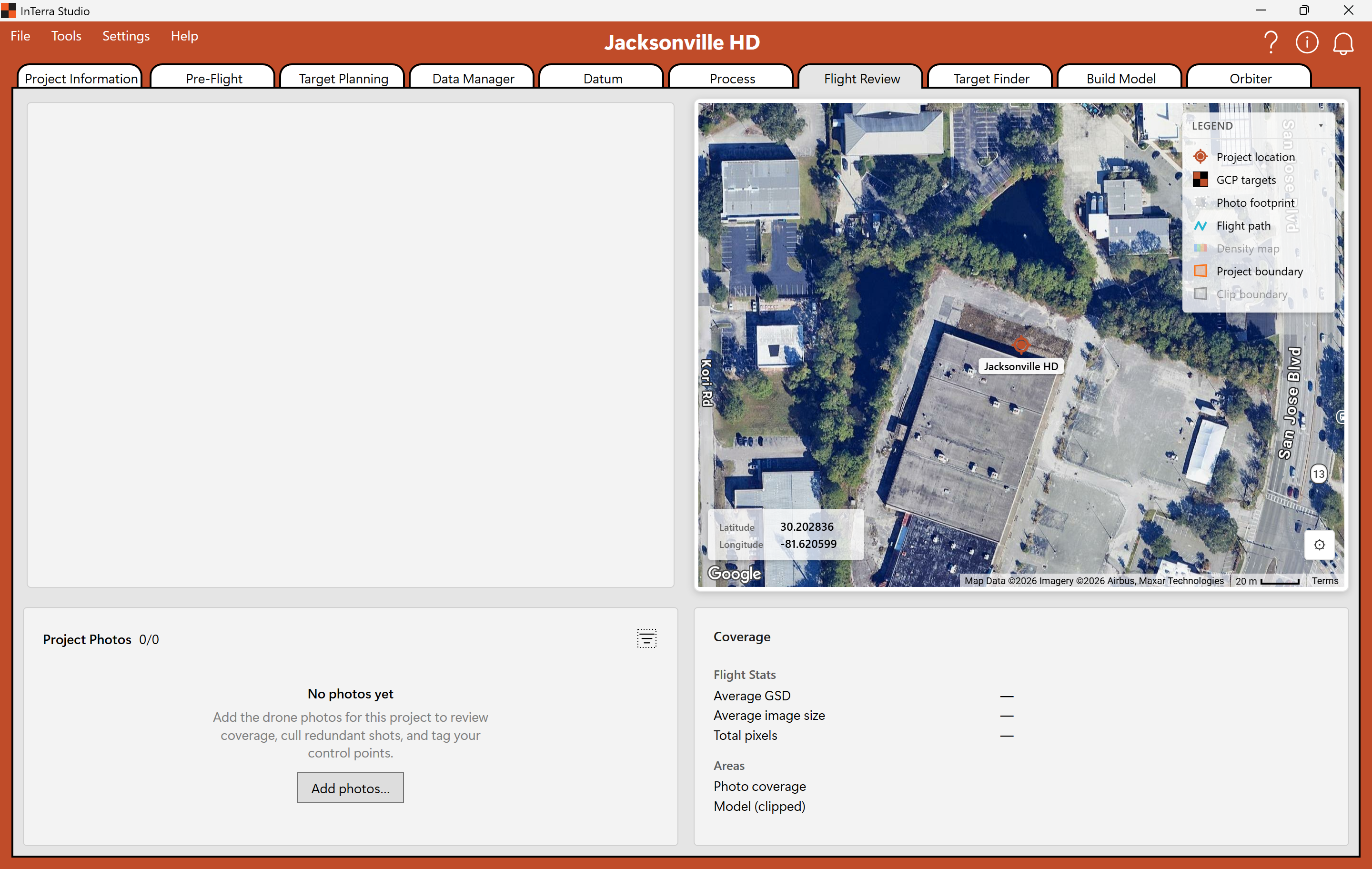
Screenshot: Flight Review before any photos are added — the empty photo panel with its Add photos… button, and the coverage statistics waiting to fill in.

Open Flight Review. With no photos yet, the photo panel shows an Add photos… button. Click it and choose the Tutorial Images folder itself — select the folder, not the files inside it. It sits beside your project, in your InTerra projects folder alongside Jacksonville HD. Then Copy them in.

The sample images are about 2 GB and download in the background from the moment you created the project, so they're normally waiting by the time you get here. If the folder is empty or short, give it a minute and look again.

Importing takes a few seconds after the copy finishes — InTerra is reading every photo's position and orientation, building its footprint, and projecting your ground control onto the imagery. The busy cursor tells you it's working; the photo list fills in when it's done.

That position data rides along in a sidecar — a small companion file written beside the photos carrying each shot's GPS position and camera angles. Some drones write everything into the images themselves and produce no sidecar at all; it depends on the aircraft and camera. Either way InTerra reads what's there, which is why the photos arrive already placed on the map.

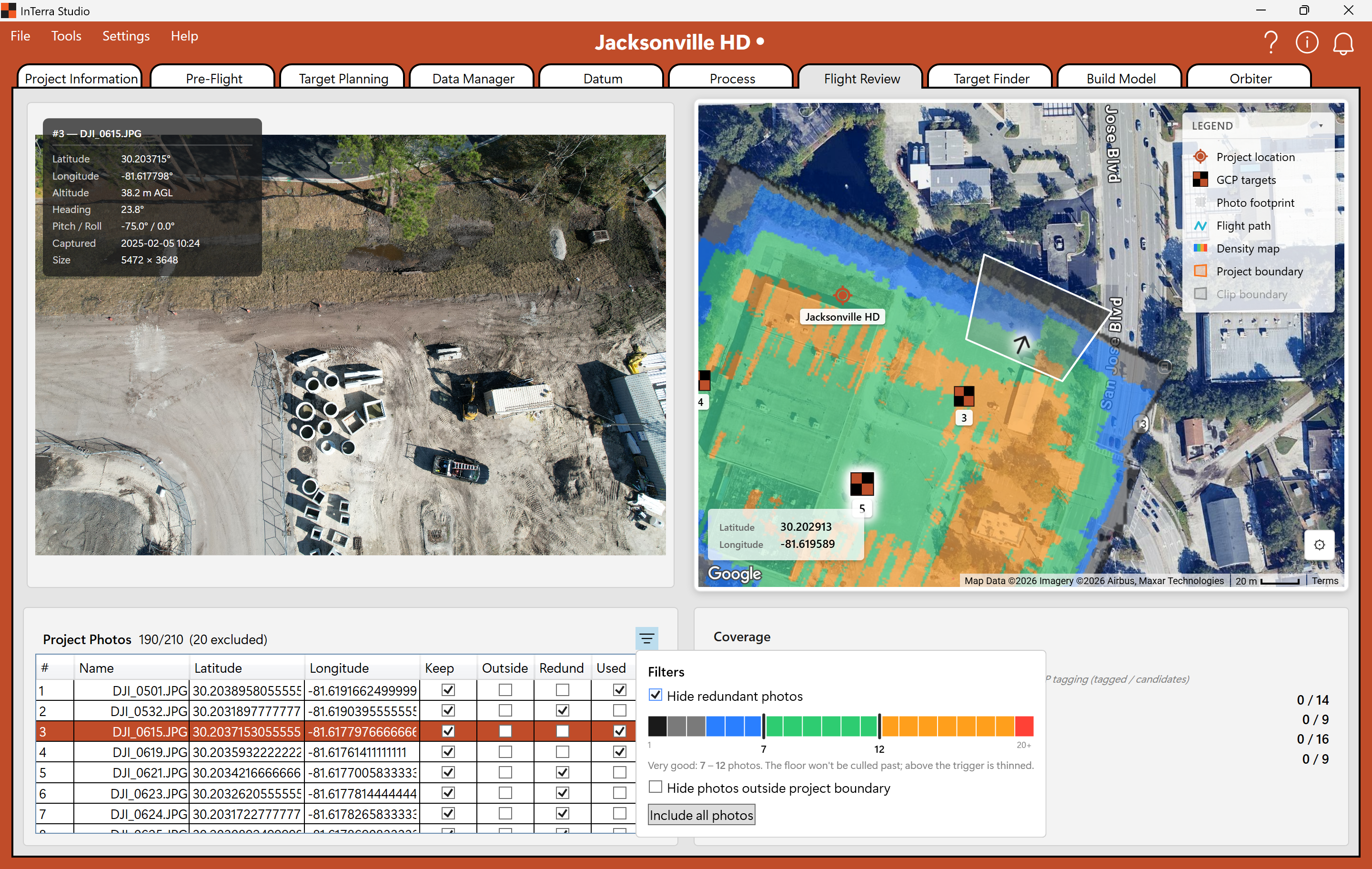
Screenshot: Flight Review with the tutorial photos imported and the density map switched on, ready to cull redundant images.

With the photos in, turn on the Density Map — open the gear in the map window and check Density Map — to see how heavily each part of the site was covered. Then run the auto-cull: open the filter to the right of Project Photos and choose Hide redundant photos.

Culling isn't only about speed. Redundant photos don't add information — the same ground from nearly the same angle tells the reconstruction nothing new, and they can actively muddy it: more chances to match the wrong feature, more weight on one over-sampled patch. Dropping them makes the build faster and cleaner, which is why coverage rather than sheer photo count is what you're aiming for. See Reference → Flight Review.

Step 7 — Tag your control (Target Finder)

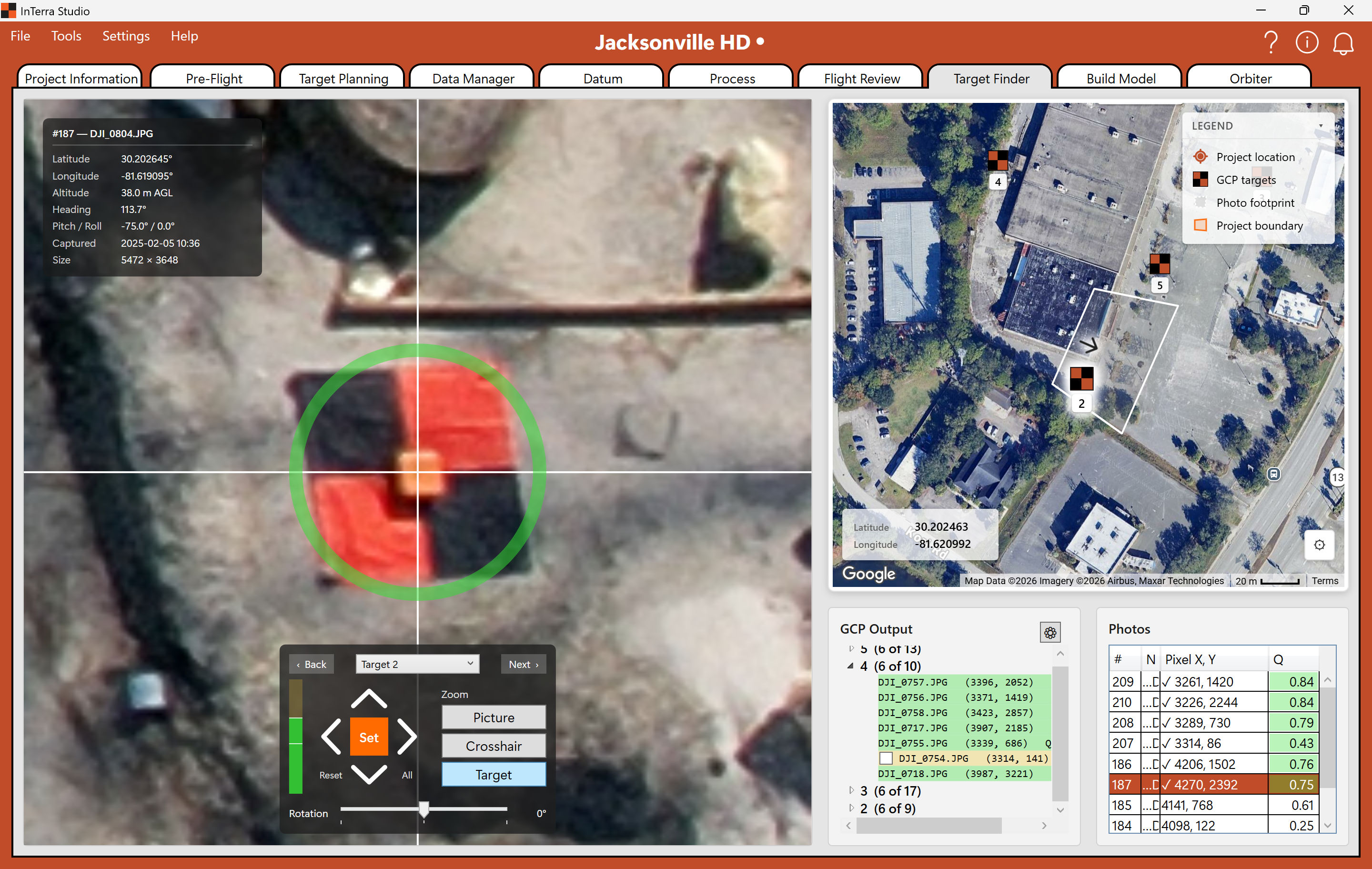
Screenshot: Target Finder with the crosshair over a ground target in one photo, the GCP tree beside it, and the candidate photo grid below.

Open Target Finder. Here you connect the ground control you computed in Step 5 to where those targets actually appear in the photos. InTerra projects each control point onto its candidate photos and shows you where it expects the target; you confirm or nudge the exact pixel.

Expect to help with the first photo of each target. On that first one InTerra has only the projected position to go on, so the crosshair may land beside the target rather than on it — nudge it onto the centre of the target and click Set Target. That first pick is what the matcher learns from: it takes the patch of image around your click and searches for it in the remaining photos, so from the second photo onward the crosshair should arrive on or very near the target and you're mostly confirming rather than hunting.

You don't need to tag every photo a target appears in. Tag four to six good photos per target, then stop — additional photos rarely add anything to the solution, and targets sitting near the edge of a frame are worth skipping. Tagging control to the imagery is what georeferences the model and drives its accuracy. See Reference → Target Finder.

Step 8 — Build the model (Build Model)

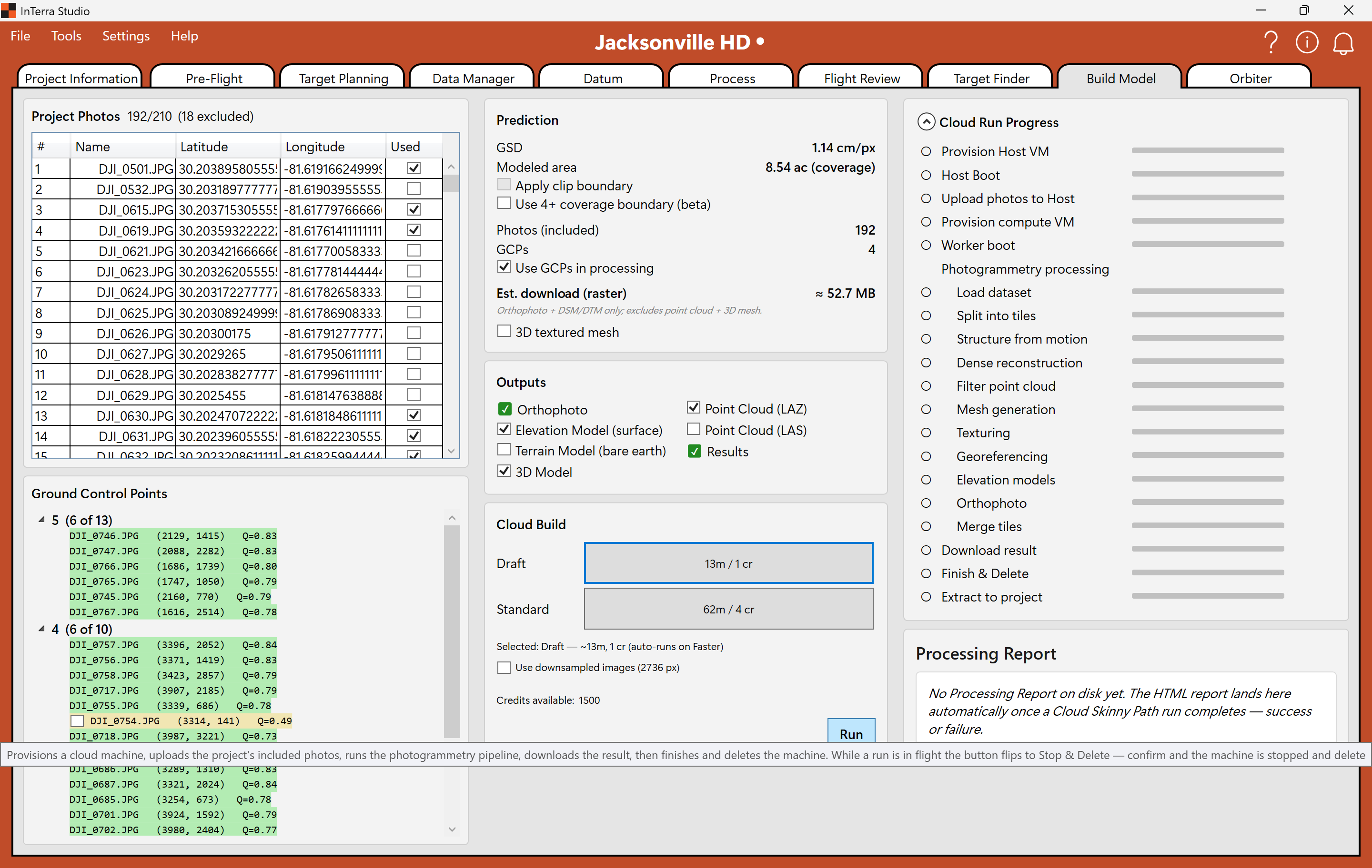
Screenshot: Build Model with the photos and ground control counted, the Draft preset selected, and its time and credit estimate showing.

Open Build Model. Choose the Draft preset and click Run.

For the tutorial, InTerra simulates the cloud build — you'll see the real processing stages run, but instantly and at no cost, and the finished deliverables drop straight into your project. On your own job this step uploads your photos to the cloud and runs the full photogrammetry pipeline (minutes to hours depending on size), then downloads the results. See Reference → Build Model.

Step 9 — Explore & measure (Orbiter)

Open Orbiter to explore your results: pan and zoom the orthophoto, orbit the 3D model, toggle the elevation and other overlays, and take a measurement. This is the deliverable your client would explore. See Reference → Orbiter.

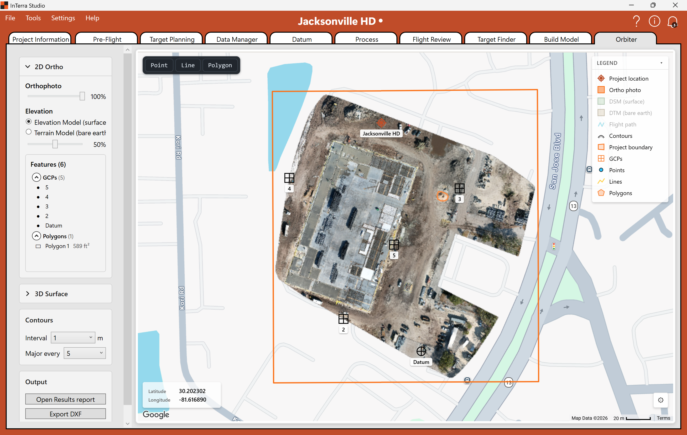
Screenshot: the finished orthophoto in Orbiter, inside the project boundary, with the tagged GCPs and the Datum shown on their own layer.

Contour colors can be controlled in Settings → Layer Colors. Now draw something: pick Polygon from the toolbar, click around a stockpile or a spoil heap, and double-click to close it.

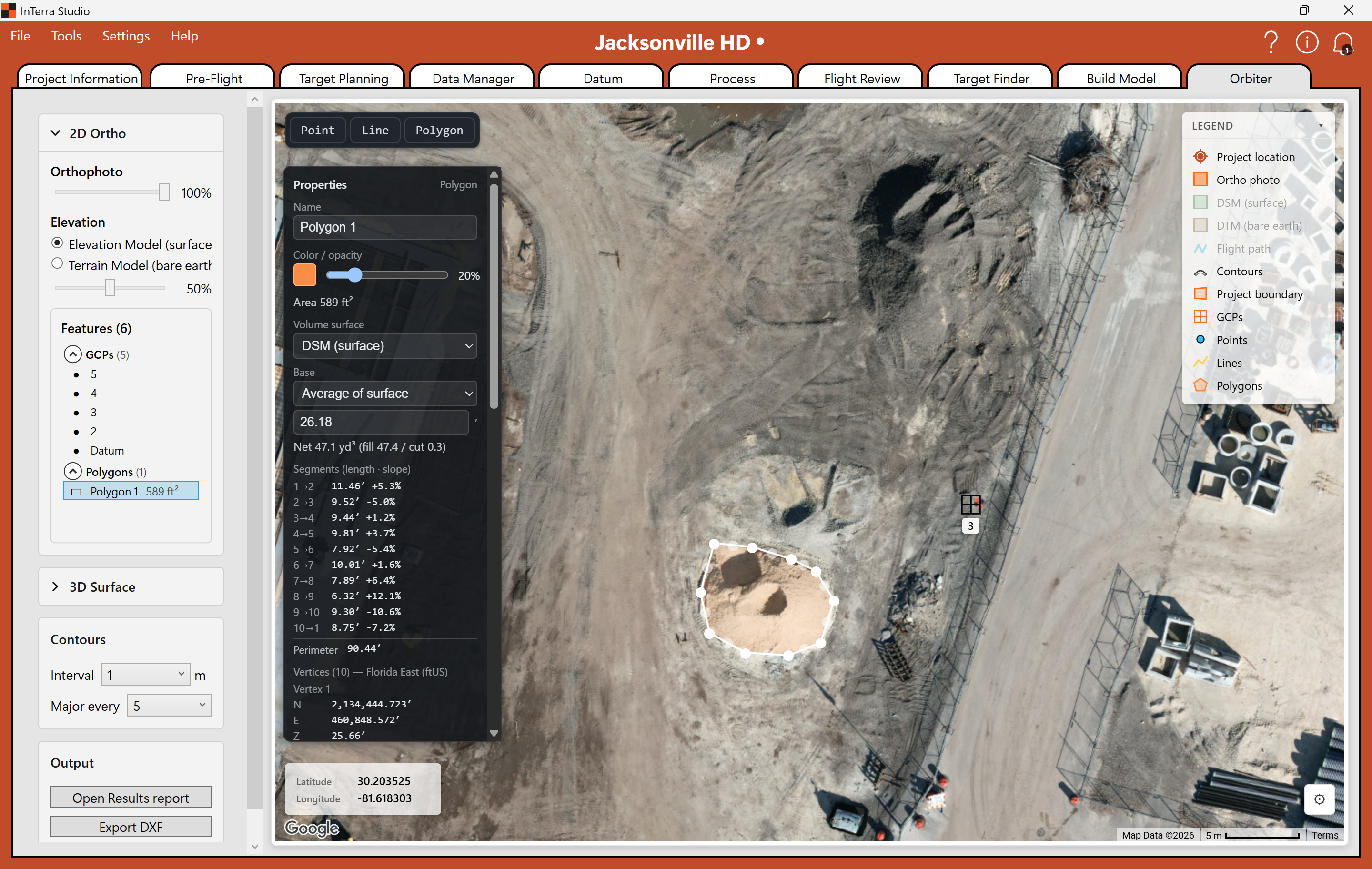
Screenshot: a drawn polygon selected on the orthophoto, its Properties card showing area, per-segment lengths and slopes, perimeter, and the volume computed against the surface model.

The Properties card fills in as soon as the shape closes: area, perimeter, per-segment length and slope, every vertex in your project's grid coordinates — and a volume, computed against the surface model with cut and fill reported separately. That's the measurement a client actually asks for, taken straight off the deliverable.

Step 10 — Your reports

InTerra generates reports from the run automatically. Open the Results report for the client-facing summary — accuracy figures, coverage, GCP residuals, and preview imagery — and the Processing report for the operator-side run diagnostics. See Reference → Reports.

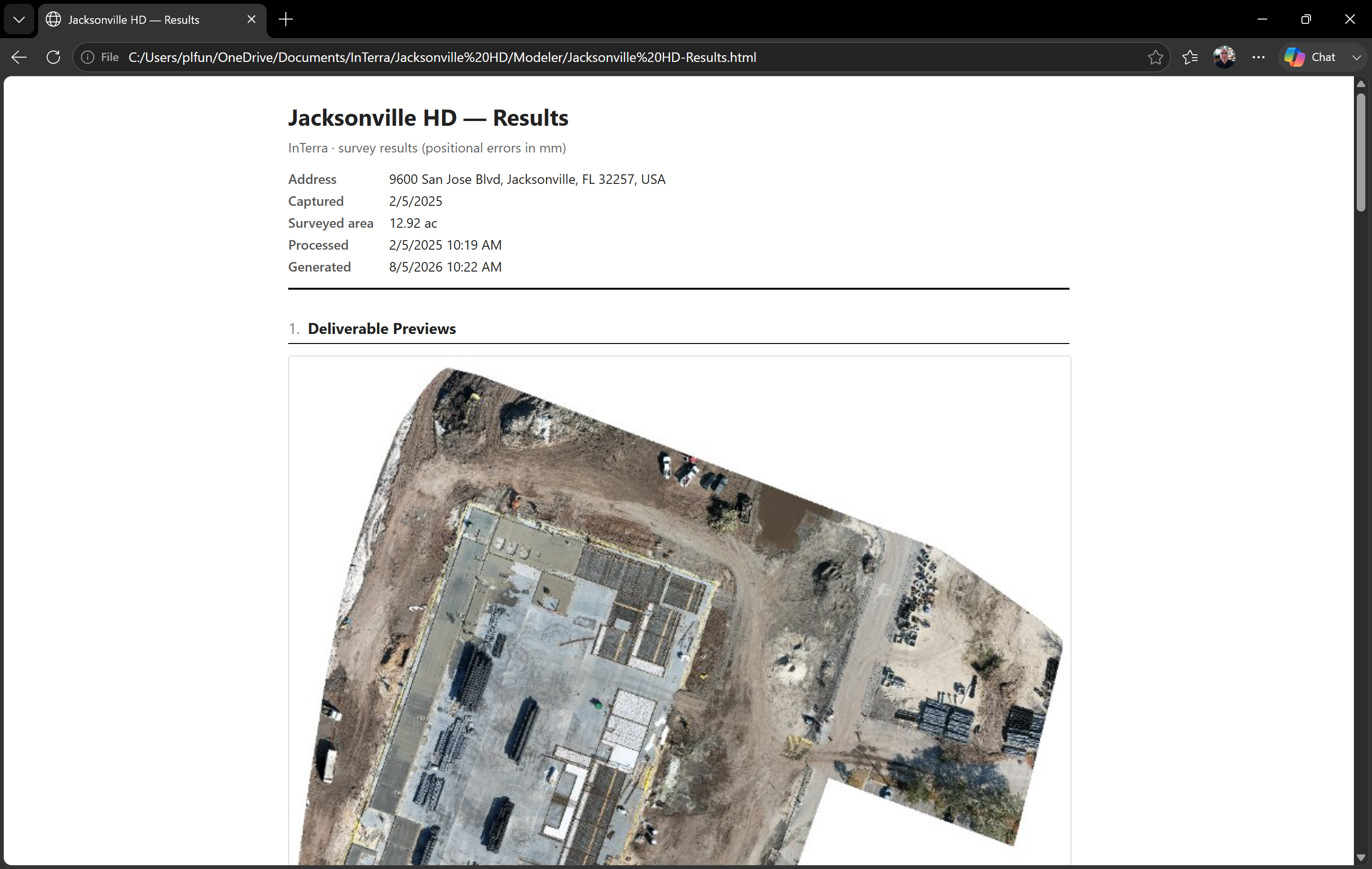
Screenshot: the client-facing Results report for the tutorial run, showing the project identity header and the accuracy summary.

What's next

You've taken a survey from an empty project all the way to a measurable 3D model. The only piece you didn't do here is the flight itself — for that, the planning tabs (Pre-Flight, Target Planning) and a field day with your SmarTargets stand in front of everything you just did.

From here, the How-to guides give step-by-step recipes for specific tasks, and the Reference has the full detail on every tab and control.